Evaluation of a Coating Process for SiO₂/TiO₂ Composite Particles by Machine Learning Techniques

Abstract

In this study, in order to optimize a fabrication process for SiO₂/TiO₂ composite particles and control their coating ratio (C_Ti), regression models for the coating process were constructed using various machine learning techniques. The composite particles with a core (SiO₂)/shell (TiO₂) structure were synthesized by mechanical stress under various fabrication conditions with respect to the supply volume of raw materials (V), addition ratio of TiO₂ (r_Ti), operation time (t), rotor rotation speed (S), and temperature (T). Regression models were constructed by the least squares method (LSM), principal component regression (PCR), support vector regression (SVR), and the deep neural network (DNN) method. The accuracy of the constructed regression models was evaluated using the determination coefficients (R²) and the predictive performance was evaluated by comparing the prediction coefficients (Q²). From the perspective of the R² and Q² values, the DNN regression model was found to be the most suitable model for the present coating process. Moreover, the effects of the fabrication parameters on C_Ti were analyzed using the constructed DNN model. The results suggested that the t value was the dominant factor determining C_Ti of the composite particles, with the plot of C_Ti versus t displaying a clear maximum.

1. Introduction

Composite particles synthesized by compounding techniques have been extensively utilized in various fields (Al-Salihi H.A. et al., 2019; Karger-Kocsis J. et al., 2014; Pierpaoli M. et al., 2019). Since powder properties play a key role in the suitability for a particular application (Kimura T. et al., 2020), selecting the optimal combination of particles is crucial for the performance of the composite particles (Deki Y. et al., 2018). For example, composite particles consisting of oxides, such as SiO₂ and TiO₂, are utilized in cosmetics and ceramics because of their superior physical properties including optical and electrical properties (Adebisi A.A. et al., 2016; Himoto I. et al., 2016). Consequently, it is necessary to control the powder properties during the fabrication of composite particles.

In the synthesis of composite particles, compounding by mixing and dispersion, which involves convection, shear, and diffusion processes, is extensively applied. These compounding techniques require a combination of impact, compression, and friction to overcome the aggregation forces. (Kim K. et al., 2016). In many cases of conventional processes using mixers and mechanical compounding machinery, premixing and compounding in other equipment is necessary because the mechanism of mixing of a single device is biased toward convection, shear, or diffusion (Thongnopkoon T. et al., 2018). Several fabrication methods for composite particles have been reported, although achieving control over the powder properties of the particles during the fabrication processes remains challenging owing to the complex relationships between the powder properties and fabrication conditions (Matsuoka Y. et al., 2021). Hence, it is essential to develop methods of predicting these complex relationships to control the powder properties of the composite particles.

Data with complex correlations are often analyzed by statistical and machine learning methods (Kaneko H. and Funatsu K., 2015; Wada S. et al., 2021; Zhao Z. et al., 2018), such as the least-squares method (LSM), principal component regression (PCR), and support vector regression (SVR) (De Backer A. et al., 2021; Tran H. et al., 2018; Zhang Z. et al., 2021). In addition, a deep neural network (DNN) analysis has proved useful in a variety of fields, including agriculture (Cai Y. et al., 2019; Qui Z. et al., 2018), environmental studies (Ghatak M.D. and Ghatak A., 2018; Tanzifi M. et al., 2018), and medicine (Basheer I.A. and Hajmeer M., 2000; Horie Y. et al., 2019; Stokes J.M. et al., 2020). DNN analysis is one of the typical machine learning methods and aims to replicate the neural circuits of the human brain by a mathematical model using multiple artificial neurons. A DNN learns by adjusting parameters in the model and can predict complex correlations (Basheer I.A. and Hajmeer M., 2000; Zhang G. et al., 1998).

In previous studies (De Backer A. et al., 2021; Tran H. et al., 2018; Zhang Z. et al., 2021), regression models were constructed to examine the relationships between several explanatory variables and the objective variables using various methods, including LSM, PCR, and SVR, and their predictive performance was improved by considering multiple explanatory variables. For example, Matsuoka et al. (Matsuoka Y. et al., 2021) investigated the relationships between the operating conditions and the physical properties of oral solid dosage tablets during a continuous manufacturing process using a DNN model, which successfully predicted the physical properties of the tablets from the operating conditions with high accuracy. In another study, regression models were constructed to estimate the volume loss of AA7075/Al₂O₃ composites during wear test at various operating conditions using the LSM, SVR, and DNN methods, and the performance of the machine learning was compared with statistical analysis for this challenging situation involving complex correlations between the explanatory and objective variables (Aydin F., 2021).

In this study, the optimization of prediction techniques for the complex correlation between powder properties and fabrication conditions by constructing regression models using several methods was investigated. Furthermore, parameters affecting the powder properties of SiO₂/TiO₂ composite particles were analyzed with a focus on the coating ratio (C_Ti) of the composite particles. The SiO₂/TiO₂ composite particles were synthesized using a powder processing system (NOB-MINI, HOSOKAWA Micron Co., Japan). Because of the balanced effects of compression, shear, and impact on individual particles, the fabrication apparatus used in this study enables particle design and particle processing, such as compounding, surface modification, and spheronization. To analyze the correlations between the fabrication conditions and C_Ti of the SiO₂/TiO₂ composite particles, the supply volume (V), addition ratio of TiO₂ (r_Ti), operation time (t), rotor rotation speed (S), and temperature (T) were varied. On the basis of the experimentally determined C_Ti values of the composite particles prepared under various fabrication conditions, regression models for C_Ti of the composite particles were obtained from the machine learning methods. Furthermore, the optimized models were used to predict C_Ti values of the composite particles under various fabrication conditions.

2. Experimental and construction methods for regression models

2.1 Materials and experimental procedure

The composite particles were prepared from SiO₂ (MT-150W, Tayca Co., Japan), as the core particle and TiO₂ (Silsic T-1 (S-1), Yamamori Tsuchimoto Inc., Japan) as the shell particle. The SiO₂ and TiO₂ particles were supplied to the experimental apparatus (NOB-MINI, HOSOKAWA Micron Co., Japan). The supply volume of the raw materials (V) and the addition ratio of TiO₂ (r_Ti) were varied in the ranges of 25–125 mL and 5.0–15.0 wt%, respectively. The operation time (t) was set to 1–15 min. The rotation speed (S) and temperature (T) were set to 2,200–5,700 min⁻¹ and 295–319 K, respectively. Under all experimental conditions, the electric current was maintained at constant value of 3.5 A. In total, the SiO₂/TiO₂ composite particles were synthesized under 29 sets of experimental conditions, as summarized in Table 1. The surface morphology of the SiO₂/TiO₂ composite particles was examined by scanning electron microscopy (SEM; SU3500 II; Hitachi High-Tech Science Co., Japan), and the Si and Ti distributions were measured using an energy-dispersive X-ray spectrometer (EDS; Ultim Max, Oxford Instruments Co., Japan) connected to the SEM. The mapping time was set at approximately 120 s. The coating ratio (C_Ti) of the composite particles was calculated according to Eqn. (1) from the integrated areas of Si (S_Si) and Ti (S_Ti) in the elemental mapping images by using imaging software (WinROOF; Mitani Corp., Japan):

  

$$C_{\text{Ti}}=\frac{S_{\text{Ti}}}{S_{\text{Si}}+S_{\text{Ti}}}$$(1)

Table 1

Summary of fabrication conditions for the SiO₂/TiO₂ composite particles.

Experimental condition
Supply volume (V) [mL]	25–125
Addition ratio of Ti (rTi) [wt%]	5.0–15.0
Operation time (t) [min]	1–15
Rotation speed (S) [min−1]	2,200–5,700
Temperature (T) [K]	295–319

2.2 Construction of regression model

The regression models were constructed as described in Sections 2.2.1–2.2.4. The fabrication parameters (V, r_Ti, t, S, and T) were employed as the explanatory variables to serve as the input values. C_Ti was chosen as the objective variable to serve as the output value. The 29 samples were split into training to construct the regression models (21 samples) and test data to evaluate the predictive performance of the constructed models (8 samples). The input and output values (z) were auto-scaled by following Eqn (2):

  

$$z^{\prime }=\frac{z-\mu }{\sigma }$$(2)

where z′ denotes the auto-scaled value, and μ and σ represent the mean and standard deviation of each explanatory variable, respectively.

The determination coefficient (R²) was used to evaluate the accuracy of the regression models constructed from the training data. The predictive performance of the constructed models was assessed by calculating the predictive coefficient (Q²) using the test data. The root mean square error (RMSE) for each model was also calculated. The formulas used to calculate the R², Q², and RMSE are given in Eqns. (3)–(5):

  

$$R^2=1-\frac{{\sum }_{i=1}^n{(y_i^{\text{calc.}}-y_i)}^2}{{\sum }_{i=1}^n{(y_{\text{mean}}-y_i)}^2}$$(3)

  

$$Q^2=1-\frac{{\sum }_{i=1}^n{(y_i^{\text{pred.}}-y_i)}^2}{{\sum }_{i=1}^n{(y_{\text{mean}}-y_i)}^2}$$(4)

  

$$\text{RMSE}=\sqrt{\frac{1}{n}\sum _{i=1}^n{(y_i^{\text{calc.},\text{pred.}}-y_i)}^2}$$(5)

where y_i, $y_i^{\text{calc.}}$, and $y_i^{\text{pred.}}$ represent the experimental value, the calculated value using the training data, and the predicted value using the test data, respectively, the subscript i denotes the i-th sample, and y_mean is the average of the experimental values.

The R² value indicates the accuracy of model construction because it expresses the degree of agreement between the experimental values and the calculated values when training data are substituted into the models constructed from training data. Meanwhile, the Q² value reflects the degree of agreement between the experimental values and the predicted values when test data are substituted into the models constructed from training data. The maximum value for both R² and Q² is 1.0, and values closer to 1.0 indicate a higher quality model. The RMSE has a positive value and is used to evaluate errors in the numerical prediction, where a smaller value indicates superior predictive performance (Barrasso D. et al., 2015).

2.2.1 Least-squares method (LSM)

LSM modeling is a construction method that involves determining the coefficients (β_LSM) that minimize the sum-of-squares error (S_LSM) between calculated values (y_calc.) and experimental values (y). When the numbers of samples and explanatory variables are m and n, respectively, the vector of error (ɛ_LSM), β_LSM, y, and matrix of explanatory variables (X) can be expressed as shown in Eqns. (6)–(9):

  

$${\mathbf{\varepsilon }}_{\mathbf{LSM}}=\left(\begin{array}{c}{\varepsilon }_{\text{LSM},\hspace{0.17em}1}\\ {\varepsilon }_{\text{LSM},\hspace{0.17em}2}\\ ⋮\\ {\varepsilon }_{\text{LSM},\hspace{0.17em}\text{m}}\end{array}\right)$$(6)

  

$${\mathit{\beta }}_{\mathbf{LSM}}=\left(\begin{array}{c}{{\beta }_{\text{LSM}}}^{(1)}\\ {{\beta }_{\text{LSM}}}^{(2)}\\ ⋮\\ {{\beta }_{\text{LSM}}}^{(n)}\end{array}\right)$$(7)

  

$$\mathit{y}=\left(\begin{array}{c}{y}_1\\ y_2\\ ⋮\\ y_m\end{array}\right)$$(8)

  

$$X=\left(\begin{array}{llll}{x_1}^{(1)}\hfill & {x_1}^{(2)}\hfill & \cdots \hfill & {x_1}^{(n)}\hfill \\ {x_2}^{(1)}\hfill & {x_2}^{(2)}\hfill & \cdots \hfill & {x_2}^{(n)}\hfill \\ \hspace{0.17em}\hfill & ⋮\hfill & \ddots \hfill & ⋮\hfill \\ {x_m}^{(1)}\hfill & {x_m}^{(2)}\hfill & \cdots \hfill & {x_m}^{(n)}\hfill \end{array}\right)$$(9)

Furthermore, the y^calc. and y vectors are given by Eqns. (10) and (11), respectively:

  

$${\mathit{y}}^{\mathbf{calc.}}=X{\mathit{\beta }}_{\mathbf{LSM}}$$(10)

  

$$\mathit{y}=X{\mathit{\beta }}_{\mathbf{LSM}}+{\mathbf{\varepsilon }}_{\mathbf{LSM}}$$(11)

Because smaller errors between the y^calc. and y vectors were desired, the β_LSM vector minimizing the S_LSM matrix, which is determined by the square sum of the ɛ_LSM vector, was sought by partial differentiation of Eqn. (11), to afford the relationship shown in Eqn. (12):

  

$$X^{\text{T}}X{\mathit{\beta }}_{\mathbf{LSM}}=X^{\text{T}}\mathit{y}$$(12)

Furthermore, when the inverse matrix of the X^TX matrix was multiplied from the left of both sides of Eqn. (12), the β_LSM vector was optimized as shown in Eqn. (13), thus constructing the LSM model:

  

$${\mathit{\beta }}_{\mathbf{LSM}}={(X^{\text{T}}X)}^{-1}{X}^{\text{T}}\mathit{y}$$(13)

For simple relationships, such as linear and quadratic functions consisting of a small number of parameters serving as explanatory variables, the LSM is a suitable method. Because the order of the explanatory variables was set to 1, the LSM model constructed in this study is a liner regression.

2.2.2 Principal component regression (PCR)

PCR modeling is a construction method in which explanatory variables are transformed into principal components that are uncorrelated with each other. The algorithm for PCR model construction consists of the following two steps (Hotelling H., 1957).

In the first step, principal component analysis (PCA) is conducted. When the score vector (t_PCR) is defined as a linear combination of the X matrix, the t_PCR vector is obtained as described by Eqn. (14):

  

$${\mathit{t}}_{\mathbf{PCR}}=X{\mathit{p}}_{\mathbf{PCR}}$$(14)

where p_PCR is the weight of the linear combination, which is referred to as loading.

Because PCA is performed by maximization of the score, the sum-of-squares score (S_PCA) is maximized by using the Lagrange multiplier (G_PCR) expressed in Eqn. (15):

  

$$\begin{array}{ll}{G}_{\text{PCR}}\hfill & =S_{\text{PCA}}-\lambda \left(\sum _{j=1}^n({(p_j)}^2-1)\right)\hfill \\ \hspace{0.17em}\hfill & =\sum _{i=1}^m{(t_i)}^2-\lambda \hspace{0.17em}\left(\sum _{j=1}^n({(p_j)}^2-1)\right)\hfill \end{array}$$(15)

where j represents the number of explanatory variables. n is the number of solutions of the equation represented by the λ value. The t_PCR vector with the n-th largest variance of λ is defined as the n-th principal component, and the principal component matrix (T) is given by Eqn. (16):

  

$$T=\left(\begin{array}{llll}{t_{\text{PCR},\hspace{0.17em}1}}^{(1)}\hfill & {t_{\text{PCR},\hspace{0.17em}2}}^{(1)}\hfill & \cdots \hfill & {t_{\text{PCR},\hspace{0.17em}n}}^{(1)}\hfill \\ {t_{\text{PCR},\hspace{0.17em}1}}^{(2)}\hfill & {t_{\text{PCR},\hspace{0.17em}2}}^{(2)}\hfill & \cdots \hfill & {t_{\text{PCR},\hspace{0.17em}n}}^{(2)}\hfill \\ \hspace{0.17em}\hfill & ⋮\hfill & \ddots \hfill & ⋮\hfill \\ {t_{\text{PCR},\hspace{0.17em}1}}^{(m)}\hfill & {t_{\text{PCR},\hspace{0.17em}2}}^{(m)}\hfill & \cdots \hfill & {t_{\text{PCR},\hspace{0.17em}n}}^{(m)}\hfill \end{array}\right)$$(16)

The PCR model was constructed by adopting the T matrix as the explanatory variables in a similar manner as described for LSM in Section 2.2.1, and the relationship between the output variables and the feature components was optimized by varying the number of principal components (N_P.C.) within the range of 1–5.

For processes with a correlation between the explanatory variables, the PCR method is considered the optimal selection because the impact of explanatory variables with dependent relationships on the accuracy of the regression model is reduced.

2.2.3 Support vector regression (SVR)

An SVR model is constructed using a support vector machine (SVM) for regression analysis. In SVR modeling, a kernel trick along with SVM is applied to construct nonlinear models. The original form of the SVR minimizes the matrix (S_SVR) shown in Eqn. (17), which is related to the vectors of error and coefficient in SVR:

  

$$S_{\text{SVR}}=\frac{1}{2}{\Vert \mathit{w}\Vert }^2+C\sum _{i=1}^N{|y_i-f({\mathit{x}}_{\mathit{i}})|}_{\varepsilon }$$(17)

where f and w denote the SVR model and a weight vector, respectively, ɛ is a threshold, C is a penalty term that controls the trade-off between the model complexity and training errors, and N is the number of training data. The second term of Eqn. (17) is the ɛ-insensitive loss function, as defined in Eqn. (18):

  

$${|y_i-f({\mathit{x}}_{\mathit{i}})|}_{\varepsilon }=\text{max\hspace{0.17em}}(0,|y_i-f\hspace{0.17em}({\mathit{x}}_{\mathit{i}})|-\varepsilon )$$(18)

Minimization of Eqn. (17) affords a regression model with a satisfactory balance between generalization capability and ability to adapt to training data. When an x vector is inputted, a y value is predicted by Eqn. (19):

  

$$y=f\hspace{0.17em}(\mathit{x})=\sum _{i=1}^N({\alpha }_i-{{\alpha }_i}^{*})\hspace{0.17em}K\hspace{0.17em}({\mathit{x}}_{\mathit{i}},\mathit{x})+u_{\text{SVR}}$$(19)

where K is a kernel function, and u_SVR is a constant. As the kernel function for this study, the radial basis function kernel given by Eqn. (20) was adopted:

  

$$K\hspace{0.17em}({\mathit{x}}_{\mathit{i}},\mathit{x})=\text{exp\hspace{0.17em}}(-\gamma \hspace{0.17em}{(\Vert {\mathit{x}}_{\mathit{i}}-\mathit{x}\Vert )}^2)$$(20)

where γ represents a turning parameter for controlling the width of the kernel function, and α_i and α_i* in Eqn. (19) are obtained from Eqns. (17) and (18) by minimizing the Lagrange multiplier (G_SVR), as expressed in Eqn. (21):

  

$$\begin{array}{ll}{G}_{\text{SVR}}=\hspace{0.17em}\hfill & \frac{1}{2}\sum _{i=1}^N\sum _{j=1}^N{K}_{ij}({\alpha }_i-{{\alpha }_i}^{*})({\alpha }_j-{{\alpha }_j}^{*})\hfill \\ \hspace{0.17em}\hfill & -\sum _{i=1}^N{y}_i({\alpha }_i-{{\alpha }_i}^{*})+\varepsilon \sum _{i=1}^N({\alpha }_i-{{\alpha }_i}^{*})\hfill \end{array}$$(21)

and the α_i and α_i* values are subject to

  

$$\{\begin{array}{l}0\le {\alpha }_i\hfill \\ {{\alpha }_j}^{*}\le C\hfill \end{array}\mathrm{\hspace{0.17em} }\mathrm{\hspace{0.17em} }\mathrm{\hspace{0.17em} }i=1,2,\dots ,N$$(22)

  

$$\sum _{i=1}^N\left({\alpha }_i-{{\alpha }_i}^{*}\right)=0$$(23)

and K_ij in Eqn. (21) is

  

$$K_{ij}=K\hspace{0.17em}\left({\mathit{x}}_{\mathit{i}},{\mathit{x}}_{\mathit{j}}\right)$$(24)

In SVR modeling, the hyperparameters (C, ɛ, and γ values) have to be set beforehand. The hyperparameters were selected by a comprehensive grid search (Kaneko H. and Funatsu K. et al., 2013).

The SVR method is suitable when it is necessary to construct a regression model to predict processes involving nonlinearities and negligible error ranges.

2.2.4 Deep neural network (DNN)

A neural network (NN) model is constructed by optimizing the hyperparameters, such as the numbers of hidden layers (N_H.L.) and neurons (N_Neur.), the activation function, and the number of learning times (N_L.T.). An NN with an N_H.L greater than two is referred to as a DNN. In this study, the N_H.L. and N_Neur. values were each varied in the range of 1–10. As the activation functions, the sigmoid function, tanh function, and rectified linear unit (ReLU) function were compared. The sigmoid function has a long history as an activation function for NN models. The tanh function has been reported to learn faster than the sigmoid function (Ismail H.Y. et al., 2019; Shirazian S. et al., 2017). In recent years, the ReLU function has seen increasing use because of several advantages such as reduced gradient vanishing and faster calculation (Roggo Y. et al., 2020). The sigmoid function, tanh function, and ReLU function are expressed in Eqns. (25), (26), and (27), respectively:

  

$$h(x)=\frac{1}{1+{\text{e}}^{-x}}$$(25)

  

$$h(x)=\frac{{\mathbf{e}}^x-{\mathbf{e}}^{-x}}{{\mathbf{e}}^x+{\mathbf{e}}^{-x}}$$(26)

  

$$h(x)=\{\begin{array}{ll}x\hfill & (x>0)\hfill \\ 0\hfill & (x\le 0)\hfill \end{array}$$(27)

In all cases, the stochastic gradient descent method was adopted as the optimization method. N_L.T. was varied in the range of 30–3,500. The hyperparameters are summarized in Table 2.

Table 2

Summary of the hyperparameter ranges used to optimize the DNN method.

Parameter
Number of hidden layers (NH.L.) [−]	1–10
Number of neurons (NNeur.) [−]	1–10
Activation function	Sigmoid Hyperbolic tangent Rectified linear unit
Loss function	Mean square error
Optimization method	Stochastic gradient descent
Learning times (NL.T.) [−]	30–3,500

For systems in which the explanatory variables and objective variables are intricately related, the DNN method is an appropriate selection.

3. Results and discussion

3.1 Fabrication of SiO₂/TiO₂ composite particles

To investigate the effects of the fabrication conditions on C_Ti of the SiO₂/TiO₂ composite particles, the particles were synthesized under 29 sets of conditions by varying the values of V (25–125 mL), r_Ti (5.0–15.0 wt%), t (1–15 min), S (2,200–5,700 min⁻¹), and T (295–319 K). V, r_Ti, t, S, and T were set to include the maximum and minimum values within the operable range of experimental manipulations. The SEM and EDS images of the SiO₂/TiO₂ composite particles for t values of 1 and 10 min are shown in Fig. 1 to demonstrate the surface morphology and the state of the TiO₂ coating on the SiO₂ particles. The V and r_Ti values were 25 mL and 5.0 wt%, respectively. The S and T values were varied with an increase in the t value. From the EDS observations, the C_Ti values of the composite particles were calculated using Eqn. (1). The data obtained from the fabrication experiments are listed in Table 3. In addition, the data subjected to auto-scaling using Eqn. (2) are listed in Table 4. During the construction of the regression models using the machine learning methods, data from 21 of the fabrication experiments were used as training data. The data from the remaining eight fabrication experiments were used as test data to evaluate the predictive performance of the constructed models.

Fig. 1

SEM and EDS images of the SiO₂/TiO₂ composite particles obtained at t values of 1 min and 10 min.

Table 3

Experimental data for the relationship between the fabrication conditions and C_Ti of the composite particles.

Run	V [mL]	rTi [wt%]	t [min]	S [min−1]	T [K]	CTi [%]
1	25	5.0	1	5,500	295	34.6
2	25	5.0	3	5,600	316	57.1
3	25	5.0	5	5,500	308	35.2
4	25	5.0	10	5,600	317	40.5
5	25	5.0	15	5,700	317	41.0
6	50	5.0	10	3,500	305	44.5
7	50	5.0	15	3,500	306	35.5
8	100	5.0	10	2,500	302	37.1
9	100	5.0	15	2,500	303	45.7
10	50	10.0	10	3,700	307	39.5
11	50	10.0	15	3,700	308	42.5
12	100	10.0	10	2,600	303	46.7
13	100	10.0	15	2,600	304	45.1
14	75	5.0	10	2,800	304	52.7
15	75	5.0	15	2,800	304	36.2
16	125	5.0	10	2,200	301	61.5
17	125	5.0	15	2,200	301	40.0
18	100	5.0	3	2,500	310	34.7
19	100	5.0	5	2,500	313	37.6
20	100	5.0	10	2,500	315	39.6
21	100	10.0	3	2,600	312	43.6
22	100	10.0	5	2,600	315	53.1
23	100	10.0	10	2,600	316	53.0
24	100	15.0	3	2,800	315	49.3
25	100	15.0	5	2,800	317	57.2
26	100	15.0	10	2,700	319	63.9
27	50	15.0	3	3,800	319	59.8
28	50	15.0	5	3,800	315	52.1
29	50	15.0	10	3,800	316	63.8

Table 4

Auto-scaled data for the relationship between the fabrication conditions and C_Ti of the composite particles.

Run	V [mL]	rTi [wt%]	t [min]	S [min−1]	T [K]	CTi [%]
1	−1.55	−0.82	−1.74	1.91	−2.24	−1.28
2	−1.55	−0.82	−1.30	2.00	0.96	1.18
3	−1.55	−0.82	−0.85	1.91	−0.34	−1.21
4	−1.55	−0.82	0.26	2.00	1.05	−0.63
5	−1.55	−0.82	1.37	2.08	1.07	−0.58
6	−0.78	−0.82	0.26	0.12	−0.74	−0.20
7	−0.78	−0.82	1.37	0.12	−0.52	−1.18
8	0.78	−0.82	0.26	−0.77	−1.20	−1.01
9	0.78	−0.82	1.37	−0.77	−1.10	−0.07
10	−0.78	0.43	0.26	0.30	−0.46	−0.75
11	−0.78	0.43	1.37	0.30	−0.20	−0.42
12	0.78	0.43	0.26	−0.68	−1.06	0.05
13	0.78	0.43	1.37	−0.68	−0.86	−0.13
14	0.00	−0.82	0.26	−0.50	−0.89	0.70
15	0.00	−0.82	1.37	−0.50	−0.86	−1.11
16	1.55	−0.82	0.26	−1.04	−1.32	1.66
17	1.55	−0.82	1.37	−1.04	−1.30	−0.69
18	0.78	−0.82	−1.30	−0.77	−0.02	−1.27
19	0.78	−0.82	−0.85	−0.77	0.43	−0.95
20	0.78	−0.82	0.26	−0.77	0.84	−0.74
21	0.78	0.43	−1.30	−0.68	0.41	−0.30
22	0.78	0.43	−0.85	−0.68	0.79	0.74
23	0.78	0.43	0.26	−0.68	0.98	0.73
24	0.78	1.68	−1.30	−0.50	0.76	0.33
25	0.78	1.68	−0.85	−0.50	1.16	1.19
26	0.78	1.68	0.26	−0.59	1.37	1.92
27	−0.78	1.68	−1.30	0.39	1.41	1.47
28	−0.78	1.68	−0.85	0.39	0.84	0.64
29	−0.78	1.68	0.26	0.39	1.02	1.91

3.2 Model construction using machine learning methods

The regression models were constructed using four machine learning methods, namely, LSM, PCR, SVR, and DNN. Regression analysis was performed to predict C_Ti of the SiO₂/TiO₂ composite particles depending on the values of V (25–125 mL), r_Ti (5.0–15.0 wt%), t (1–15 min), S (2,200–5,700 min⁻¹), and T (295–319 K), which were input as explanatory variables. C_Ti of the composite particles was set as the objective variable to serve as the output value. The accuracy of the constructed regression models with respect to the training data was evaluated by calculating the R² values according to Eqn. (3), and the predictive performances of the constructed models with respect to the test data were compared using the Q² values calculated from Eqn. (4). The errors of the regression models were evaluated by calculating the RMSE values according to Eqn. (5).

3.2.1 Construction of the LSM model

The LSM model represents the relationship between the explanatory variables and objective variable (Stojanovic B. et al., 2016). When the order of the explanatory variables is 1, as in this study, the relationship derived by the LSM is linear. Thus, the regression model constructed by the LSM according to Eqns. (6)–(13) is expressed in Eqn. (28):

  

$${C_{\text{Ti}}}^{\prime }=0.0669V^{\prime }+0.616{r_{\text{Ti}}}^{\prime }+0.0215t^{\prime }+0.0532S^{\prime }+0.242T^{\prime }$$(28)

where V′, r_Ti′, t′, S′, and T′ denote the auto-scaled values of each fabrication parameter and C_Ti′ is the auto-scaled value of C_Ti of the SiO₂/TiO₂ composite particles. Hence the coefficients in Eqn. (28) reflect the influence of the corresponding parameter on C_Ti of the composite particles. All of the coefficients were positive, indicating that increasing the value of each fabrication parameter increased C_Ti of the composite particles. Furthermore, the contribution of each parameter to C_Ti of the composite particles was calculated by comparing the absolute values of the coefficients. The contributions of the parameters decreased in the following order: r_Ti (61.6 %) > T (24.2 %) > V (6.69 %) > S (5.32 %) > t (2.15 %).

The relationship between the actual C_Ti values obtained from the experimental data and the calculated values obtained from the LSM regression model is presented in Fig. 2. The input values were 0.617 and 5.99 %, respectively. In general, the accuracy of a constructed regression model increases as the R² value approaches 1.0 and the RMSE value decreases. The low R² value was attributed to the features of LSM.

Fig. 2

Relationship between the actual and predicted C_Ti values for the LSM regression model.

The correlation represented by the LSM is a linear variation of C_Ti of the composite particles with respect to five fabrication parameters (Arioli M. and Gratton S., 2012; Zhang Y. and Fearn T., 2015). Thus, when the correlation between the fabrication parameters and C_Ti of the composite particles is not linear, this nonlinear relationship cannot be adequately expressed by a regression model based on the LSM (Arioli M. and Gratton S., 2012; Zhang Y. and Fearn T., 2015). Moreover, if the fabrication parameters are highly related to each other, the coefficients in Eqn. (28) could be anomalous owing to instability in the analytical calculations and the inaccuracy of the regression equation (Arioli M. and Gratton S., 2012; Zhang Y. and Fearn T., 2015).

3.2.2 Construction of the PCR model

In an effort to deal with the inaccuracy and instability of the regression model due to the correlation between the fabrication parameters as described in Section 3.2.1, the parameters were converted to principal components uncorrelated with each other by using PCA as expressed in Eqns. (14) and (15). Because the fabrication parameters highly related to each other were removed in advance, this allowed for prediction of C_Ti of the composite particles by a combination of fabrication parameters with low correlation (El Ghaziri A. and Qannari E.M., 2015).

The number of principal components (N_P.C.) was varied within the range of 1–5, and the relationship between the actual C_Ti values obtained from the experimental data and the calculated values obtained from the PCR regression models for different N_P.C. values are presented in Fig. 3. The R² values for each regression model are also indicated. When the data points are closer to the dotted line of y = x in the plots, the R² values for the PCR regression models approach 1.0. Because the R² values increased with increasing N_P.C., all five of principal components were applied to the construction of the PCR regression model.

Fig. 3

Actual and predicted C_Ti values for the PCR regression model with various N_P.C. values.

The PCR regression model constructed with N_P.C. of 5 is expressed in Eqn. (29):

  

$$C_{\text{Ti}}=0.635t_{\text{PCR},1}+0.249t_{\text{PCR},2}+0.0690t_{\text{PCR},3}+0.0549t_{\text{PCR},4}+0.0221t_{\text{PCR},5}$$(29)

where t_PCR,i represents the i-th principal component obtained by PCA. The effects of the principal components on C_Ti of the composite particles are expressed by each coefficient. The obtained R² and RMSE values were 0.617 and 5.99 %, respectively. The fact that all of the principal components were applied to the construction of the regression model implies that the correlation between each fabrication parameter prior to PCR processing was not strong (El Ghaziri A. and Qannari E.M., 2015).

When all of the principal components were used to construct the regression model, the values calculated from the PCR regression model were identical to those calculated from the LSM model, because the application of the last principal component means that any effect of the fabrication parameters was not removed. Hence, the contribution of any correlation between the fabrication parameters to the low accuracy of the LSM regression model discussed in Section 3.2.1 was small. Thus, in an attempt to improve the accuracy of the regression models, we next considered the possibility of a nonlinear correlation between the fabrication parameters and C_Ti of the composite particles.

3.2.3 Construction of SVR model

To consider a nonlinear correlation between the fabrication parameters and C_Ti of the composite particles, a regression model was constructed using SVR according to Eqns. (17)–(24). Regression models using SVR are constructed by minimizing the structural risk. The hyperparameters (C, ɛ, and γ) of the SVR model were optimized by adapting the comprehensive combination from the candidates listed in Table 5 by exploring hyperparameters with maximum R² values in verification results. The C, ɛ, and γ values in the optimized SVR model were 2⁻⁵, 2⁰, and 2⁻², respectively.

Table 5

Hyperparameters used in the SVR regression model.

C	2−5, 2−4, …, 29, 210	16 candidates
ɛ	2−15, 2−14, …, 2−1, 20	16 candidates
γ	2−20, 2−19, …, 29, 210	31 candidates

The relationship between the actual C_Ti values obtained from the experimental data and the calculated values obtained from the SVR regression model is shown in Fig. 4. The R² and RMSE values were 0.591 and 5.80 %, respectively. The former value is slightly lower than that obtained for the LSM model (0.617), indicating a lower accuracy. In contrast, the RMSE value was slightly smaller for the SVR model, indicating a high accuracy.

Fig. 4

Relationship between the actual and predicted C_Ti values for the SVR regression model.

This comparison based on the R² and RMSE values suggests that the SVR and LSM models had similar accuracy. Thus, under the conditions of this study, consideration of the possibility of a nonlinear correlation between the fabrication parameters and C_Ti of the composite particles resulted in little change in the accuracy of the regression model. Therefore, we next considered the possibility of more complex correlations between the fabrication parameters and C_Ti of the composite particles.

3.2.4 Construction of DNN model

To consider more complex correlations between the fabrication parameters and C_Ti of the composite particles, a regression model was constructed using a DNN. For this model, the hyperparameters (N_H.L., N_Neur., activation function and N_L.T.) were optimized by exploring which hyperparameters afford the highest R₂ values in the verification results.

The variation of the R² values with N_H.L., N_Neur., and N_L.T. is plotted in Fig. 5. In the case of N_H.L., as shown in Fig. 5a), the R² values were almost constant for N_H.L. values in the ranges of 1–5 layers and 6–10 layers but increased slightly when N_H.L. was increased from 5 layers to 6 layers. This increase in the R² values with an increase in N_H.L. from 5 layers to 6 layers is caused by improved fit of the relation between the fabrication parameters and C_Ti of the composite particles. In the case of N_Neur., as shown in Fig. 5b), the R² values tended to increase with increasing N_Neur. in the range of 1–6 neurons, after which the R² values remained almost constant irrespective of N_Neur.. This increase in the R² values with increasing N_Neur. in the range of 1–6 neurons is caused by improved fit of the relation between the fabrication parameters and C_Ti of the composite particles. The minimal variation of the R² values in the N_Neur. range of 6–10 neurons was attributable to the sufficiently good fit at the N_Neur. of 6 neurons. Finally, N_L.T. was varied in the range of 30–3,500 times. As shown in Fig. 5c), the R² values rapidly increased as N_L.T. was increased from 30 to 700 times. Then, as N_L.T. was increased from 700 to 1,500 times, the R² values increased more gradually. At N_L.T. values above 1,500, the R² values remained almost constant irrespective of N_L.T.. Comparison of various activation functions revealed that the tanh afforded the highest R² value, as summarized in Table 6. Hence, the optimized hyperparameters for the DNN regression model were an N_H.L. of six layers, an N_Neur. of six neurons, an N_L.T. of 1,500 times, and a tanh activation function.

Fig. 5

R² values with variation in a) N_H.L., b) N_Neur., and c) N_L.T. for optimizing the DNN regression model.

Table 6

Relationship between the R² values and activation functions for optimizing the DNN regression model.

Activation function	R2 [−]
Sigmoid	0.0294
tanh	0.596
ReLU	0.152

The relationship between the actual C_Ti values obtained from the experimental data and the calculated values obtained from the DNN regression model is plotted in Fig. 6. The R² and RMSE values were 0.941 and 2.19 %, respectively. Comparison of the results obtained for the DNN, LSM, and SVR regression models revealed that the DNN model displayed the highest accuracy, as indicated by its high R² value and low RMSE value.

Fig. 6

Relationship between the actual and predicted C_Ti values for the DNN regression model.

3.3 Comparison of constructed models

The LSM, PCR, SVR, and DNN regression models were used to predict C_Ti of the SiO₂/TiO₂ composite particles under various fabrication conditions based on the test data. Moreover, the predictive performances of the constructed models were evaluated by comparison of their Q²-values.

The relationship between the actual C_Ti values obtained from the experimental data and the calculated values obtained from the LSM, SVR, and DNN models for the training data are plotted in Fig. 7. Furthermore, to verify the predictive performances of the constructed models, the relationships between the actual C_Ti values obtained from the experimental data and the predicted values obtained from the three models for the test data are shown in Fig. 8. The results for the PCR regression model are excluded from these plots because they were identical to these obtained from the LSM model. The horizontal and vertical axes show the actual values obtained from the experimental data and the predicted values calculated from the training data or test data, respectively. The R² and Q² values become closer to 1.0 as the data points approach the dotted line of y = x in the plots. The R² and Q² values for each regression model are summarized in Table 7, along with the RMSE values for the training data (RMSE_train) and test data (RMSE_test).

Fig. 7

Comparison of the accuracy of the various regression models by R² values based on the training data.

Fig. 8

Comparison of the predictive performance of the various regression models by Q² values based on the test data.

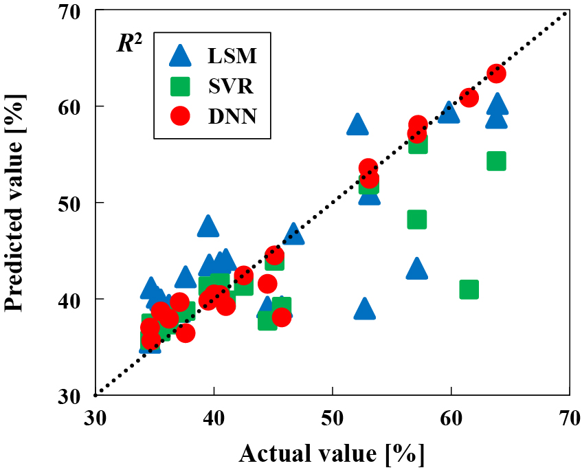
Table 7

Summary of the R², Q₂, and RMSE values for the various regression models.

	R2 [−]	RMSEtrain [%]	Q2 [−]	RMSEtest [%]
LSM	0.617	5.99	−0.510	9.28
SVR	0.591	5.80	0.280	7.97
DNN	0.941	2.19	0.767	3.26

Comparison of the R² values for the three regression models revealed that the DNN model had the highest accuracy. Similarly, the DNN model displayed the highest Q² value, indicating the best predictive performance. For a regression model with high accuracy and predictive performance, higher R² and Q² values are required (Gurgenc T. et al., 2020). The high R² and Q² values of 0.941 and 0.767 obtained for the DNN regression model in this study demonstrate the successful construction of a regression model with high accuracy and predictive performance for estimating C_Ti of SiO₂/TiO₂ composite particles. The RMSE values for the training data and test data were 2.19 % and 3.26 %, respectively. The average C_Ti of the SiO₂/TiO₂ composite particles in the experimental data was 46.3 %. In comparison, the RMSE values for the training and test data were sufficiently small. Thus, the construction of a regression model for predicting C_Ti of SiO₂/TiO₂ composite particles under various fabrication conditions was successfully realized by using the DNN method.

The DNN regression model displayed the highest accuracy in this study because the DNN method considers more complex correlations between explanatory variables and objective variables, including nonlinearities, by varying N_H.L. and N_Neur.. The LSM regression model attempts to predict the C_Ti values by calculating a formula based on simple relationships involving the explanatory variables. Meanwhile, the PCR regression model has similar features to the LSM model because the main difference between the two methods is the replacement of explanatory valuables with principal components. The SVR regression model is constructed by using explanatory variables converted to support vectors by processing with kernel functions. Because the support vectors of SVR models are used in the same manner as the principal components of PCR models, SVR models possess similar characteristics to LSM and PCR models. Therefore, the constructed SVR regression model also predicted the C_Ti values from a calculation formula involving only simple relationships. In contrast, the application of the DNN method to construct a regression model leads to predictions based on complex correlations between the explanatory variables and objective variables because of the numerous hidden layers and neurons inherent to this approach.

3.4 Analyzing the effects of fabrication conditions on C_Ti of SiO₂/TiO₂ composite particles by the DNN regression model

The DNN regression model was applied to analyzed the relationship between the fabrication conditions and C_Ti of the SiO₂/TiO₂ composite particles. The application range of the DNN regression model with respect to the five fabrication parameters was V = 25–125 mL, r_Ti = 5.0–15.0 wt%, t = 1–15 min, S = 2,200–5,700 min⁻¹, and T = 295–320 K. Each fabrication parameter serving as an input value was divided into 20 points over the corresponding range, and C_Ti of the SiO₂/TiO₂ composite particles was predicted using the DNN regression model.

The calculated effects of the fabrication parameters on C_Ti of the SiO₂/TiO₂ composite particles are plotted in Fig. 9. Comparison of the resulting curves revealed that the maximum gradients decreased in the following order: t > T > V > r_Ti > S. Because a higher gradient indicates a larger influence of the fabrication parameter on C_Ti of the composite particles, these results suggest that the effects of the fabrication parameters on C_Ti decrease in the same order. The V, r_Ti, t, S and T values under the base condition when varying each parameter were 100 mL, 5.0 wt%, 5 min, 2,500 min⁻¹, and 303 K, respectively.

Fig. 9

Calculated effects of the fabrication parameters on C_Ti of the composite particles.

The plot of C_Ti versus t revealed a clear maximum. C_Ti of the composite particles initially increased with increasing t owing to the gradual coating of TiO₂ onto SiO₂ over time. However, at higher t values, C_Ti of the composite particles decreased as a result of exfoliation of the surface coating.

Upon varying T, C_Ti of the composite particles markedly decreased with increasing T in the low-T range then remained almost constant with increasing T in the high T range. These findings suggest that lower T values are beneficial for enhancing C_Ti of SiO₂/TiO₂ composite particles.

The variation of V initially had little effect on C_Ti of the composite particles, which remained almost constant with increasing V in the low-V range. At higher values of V, C_Ti of the composite particles decreased with increasing V, which was ascribed to a decrease in the contact frequency per single particle.

Examining of the relationship between r_Ti and C_Ti of the composite particles revealed that C_Ti slightly decreased with increasing r_Ti at lower r_Ti values. However, at higher r_Ti values, C_Ti increased with increasing r_Ti, which was attributed to the increased proportion of TiO₂ particles with respect to SiO₂.

Finally, upon increasing S, C_Ti of the composite particles slightly increased. This was ascribed to the progress of coating TiO₂ onto SiO₂.

4. Conclusion

In this study, SiO₂/TiO₂ composite particles with different C_Ti values were synthesized under various conditions (V, r_Ti, t, S, and T). To optimize the fabrication process of SiO₂/TiO₂ composite particles, regression models were constructed to predict C_Ti of the composite particles using the LSM, PCR, SVR, and DNN approaches. Furthermore, the regression model with the highest accuracy and predictive performance was employed to analyze the effects of the fabrication parameters on C_Ti of the SiO₂/TiO₂ coated composite particles. The obtained results can be summarized as follows:

• 1)    SiO₂/TiO₂ composite particles were fabricated by coating TiO₂ onto SiO₂ at various V, r_Ti, t, S, and T values.
• 2)    Comparison of the constructed regression models with respect to the training data revealed that the DNN regression model displayed the highest accuracy.
• 3)    Comparison of the constructed regression models with respect to the test data indicated that the DNN regression model exhibited the best predictive performance.
• 4)    Analysis of the effects of the fabrication parameters on C_Ti of the SiO₂/TiO₂ composite particles using the DNN regression model revealed that t was the most influential factor governing C_Ti of the SiO₂/TiO₂ composite particles.

Acknowledgement

This study was financially supported by the HOSOKAWA Powder Technology Foundation (No. 20502), Osaka, Japan.

References

•  Adebisi  A.A.,  Maleque  M.A.,  Ali  M.Y.,  Bello  K.A., Effect of variable particle size reinforcement on mechanical and wear properties of 6061Al–SiCp composite, Composite Interfaces, 23 (2016) 533–547. DOI:10.1080/09276440.2016.1167414
•  Al-Salihi  H.A.,  Mahmood  A.A.,  Alalkawi  H.J., Mechanical and wear behavior of AA7075 aluminum matrix composites reinforced by Al₂O₃ nanoparticles, Nanocomposites, 5 (2019) 67–73. DOI:10.1080/20550324.2019.1637576
•  Arioli  M.,  Gratton  S., Linear regression models, least-squares problems, normal equations, and stopping criteria for the conjugate gradient method, Computer Physics Communications, 183 (2012) 2322–2336. DOI:10.1016/j.cpc.2012.05.023
•  Aydin  F., The investigation of the effect of particle size on wear performance of AA7075/Al₂O₃ composites using statistical analysis and different machine learning methods, Advanced Powder Technology, 32 (2021) 445–463. DOI:10.1016/j.apt.2020.12.024
•  De Backer  A.,  Becquart  C.S.,  Olsson  P.,  Domain  C., Modelling the primary damage in Fe and W: influence of the short-range interactions on the cascade properties: Part 2 – multivariate multiple linear regression analysis of displacement cascades, Journal of Nuclear Materials, 549 (2021) 152887. DOI:10.1016/j.jnucmat.2021.152887
•  Barrasso  D.,  El Hagrasy  A.,  Litster  J.D.,  Ramachandran  R., Multi-dimensional population balance model development and validation for a twin screw granulation process, Powder Technology, 270 (2015) 612–621. DOI:10.1016/j.powtec.2014.06.035
•  Basheer  I.A.,  Hajmeer  M., Artificial neural networks: fundamentals, computing, design, and application, Journal of Microbiological Methods, 43 (2000) 3–31. DOI:10.1016/S0167-7012(00)00201-3
•  Cai  Y.,  Guan  K.,  Lobell  D.,  Potgieter  A.B.,  Wang  S.,  Peng  J.,  Xu  T.,  Asseng  S.,  Zhang  Y.,  You  L.,  Peng  B., Integrating satellite and climate data to predict wheat yield in Australia using machine learning approaches, Agricultural and Forest Meteorology, 274 (2019) 144–159. DOI:10.1016/j.agrformet.2019.03.010
•  Deki  Y.,  Kadota  K.,  Onda  S.,  Tozuka  Y.,  Shimosaka  A.,  Yoshida  M.,  Shirakawa  Y., Crystallization behavior of glycine molecules with electrolytic dissociation on charged silica gel particles, Chemical Engineering & Technology, 41 (2018) 1073–1079. DOI:10.1002/ceat.201700398
•  Ghatak  M.D.,  Ghatak  A., Artificial neural network model to predict behavior of biogas production curve from mixed lignocellulosic co-substrates, Fuel, 232 (2018) 178–189. DOI:10.1016/j.fuel.2018.05.051
•  El Ghaziri  A.,  Qannari  E.M., A continuum standardization of the variables. Application to principal components analysis and PLS-regression, Chemometrics and Intelligent Laboratory Systems, 148 (2015) 95–105. DOI:10.1016/j.chemolab.2015.09.008
•  Gurgenc  T.,  Altay  O.,  Ulas  M.,  Ozel  C., Extreme learning machine and support vector regression wear loss predictions for magnesium alloys coated using various spray coating methods, Journal of Applied Physics, 127 (2020) 185103. DOI:10.1063/5.0004562
•  Himoto  I.,  Yamashita  S.,  Kita  H., Design of heat emission controlled spherical container constructed with skeletal ceramic units based on heat transfer analysis, Journal of Chemical Engineering of Japan, 49 (2016) 850–863. DOI:10.1252/jcej.15we122
•  Horie  Y.,  Yoshio  T.,  Aoyama  K.,  Yoshimizu  S.,  Horiuchi  Y.,  Ishiyama  A.,  Hirasawa  T.,  Tsuchida  T.,  Ozawa  T.,  Ishihara  S.,  Kumagai  Y.,  Fujishiro  M.,  Maetani  I.,  Fujisaki  J.,  Tada  T., Diagnostic outcomes of esophageal cancer by artificial intelligence using convolutional neural networks, Gastrointestinal Endoscopy, 89 (2019) 25–32. DOI:10.1016/j.gie.2018.07.037
•  Hotelling  H., The relations of the newer multivariate statistical methods to factor analysis, British Journal of Statistical Psychology, 10 (1957) 69–79. DOI:10.1111/j.2044-8317.1957.tb00179.x
•  Ismail  H.Y.,  Singh  M.,  Darwish  S.,  Kuhs  M.,  Shirazian  S.,  Croker  D.M.,  Khraisheh  M.,  Albadarin  A.B.,  Walker  G.M., Developing ANN-Kriging hybrid model based on process parameters for prediction of mean residence time distribution in twin-screw wet granulation, Powder Technology, 343 (2019) 568–577. DOI:10.1016/j.powtec.2018.11.060
•  Kaneko  H.,  Funatsu  K., Nonlinear regression method with variable region selection and application to soft sensors, Chemometrics and Intelligent Laboratory Systems, 121 (2013) 26–32. DOI:10.1016/j.chemolab.2012.11.017
•  Kaneko  H.,  Funatsu  K., Fast optimization of hyperparameters for support vector regression models with highly predictive ability, Chemometrics and Intelligent Laboratory Systems, 142 (2015) 64–69. DOI:10.1016/j.chemolab.2015.01.001
•  Kim  K.,  Kim  J., Core-shell structured BN/PPS composite film for high thermal conductivity with low filler concentration, Composites Science and Technology, 134 (2016) 209–216. DOI:10.1016/j.compscitech.2016.08.024
•  Kimura  T.,  Wada  Y.,  Kamei  S.,  Shirakawa  Y.,  Hiaki  T.,  Matsumoto  M., Synthesis of CaMg(CO₃)₂ from concentrated brine by CO₂ fine bubble injection and conversion to inorganic phosphor, Journal of Chemical Engineering of Japan, 53 (2020) 555–561. DOI:10.1252/jcej.20we034
•  Karger-Kocsis  J.,  Bárány  T., Single-polymer composites (SPCs): status and future trends, Composites Science and Technology, 92 (2014) 77–94. DOI:10.1016/j.compscitech.2013.12.006
•  Matsuoka  Y.,  Ohsaki  S.,  Nakamura  H.,  Watano  S., Analysis of continuous manufacturing process of oral solid dosage using neural network, Journal of the Society of Powder Technology, Japan, 58 (2021) 414–423. DOI:10.4164/sptj.58.414
•  Pierpaoli  M.,  Zheng  X.,  Bondarenko  V.,  Fava  G.,  Ruello  M.L., Paving the way for a sustainable and efficient SiO₂/TiO₂ photocatalytic composite, Environments, 6 (2019) 87–98. DOI:10.3390/environments6080087
•  Qui  Z.,  Chen  J.,  Zhao  Y.,  Zhu  S.,  He  Y.,  Zhang  C., Variety identification of single rice seed using hyperspectral imaging combined with convolutional neural network, Applied Sciences, 8 (2018) 212. DOI:10.3390/app8020212
•  Roggo  Y.,  Jelsch  M.,  Heger  P.,  Ensslin  S.,  Krumme  M., Deep learning for continuous manufacturing of pharmaceutical solid dosage form, European Journal of Pharmaceutics and Biopharmaceutics, 153 (2020) 95–105. DOI:10.1016/j.ejpb.2020.06.002
•  Shirazian  S.,  Kuhs  M.,  Darwish  S.,  Croker  D.,  Walker  G.M., Artificial neural network modelling of continuous wet granulation using a twin-screw extruder, International Journal of Pharmaceutics, 521 (2017) 102–109. DOI:10.1016/j.ijpharm.2017.02.009
•  Stojanović  B.,  Babić  M.,  Veličković  S.,  Blagojević  J., Tribological behavior of aluminum hybrid composites studied by application of factorial techniques, Tribology Transactions, 59 (2016) 522–529. DOI:10.1080/10402004.2015.1091535
•  Stokes  J.M.,  Yang  K.,  Swanson  K.,  Jin  W.,  Cubillos-Ruiz  A.,  Donghia  N.M.,  MacNair  C.R.,  French  S.,  Carfrae  L.A.,  Bloom-Ackermann  Z.,  Tran  V.M.,  Chiappino-Pepe  A.,  Badran  A.H.,  Andrews  I.W.,  Chory  E.J., et al.., A deep learning approach to antibiotic discovery, Cell, 180 (2020) 688–702.e13. DOI:10.1016/j.cell.2020.01.021
•  Tanzifi  M.,  Yaraki  M.T.,  Kiadehi  A.D.,  Hosseini  S.H.,  Olazar  M.,  Bharti  A.K.,  Agarwal  S.,  Gupta  V.K.,  Kazemi  A., Adsorption of Amido Black 10B from aqueous solution using polyaniline/SiO₂ nanocomposite: Experimental investigation and artificial neural network modeling, Journal of Colloid and Interface Science, 510 (2018) 246–261. DOI:10.1016/j.jcis.2017.09.055
•  Thongnopkoon  T.,  Chittasupho  C., Curcumin composite particles prepared by spray drying and in vitro anti-cancer activity on lung cancer cell line, Journal of Drug Delivery Science and Technology, 45 (2018) 397–407. DOI:10.1016/j.jddst.2018.04.006
•  Tran  H.,  Kim  J.,  Kim  D.,  Choi  M.,  Choi  M., Impact of air pollution on cause-specific mortality in Korea: results from Bayesian model averaging and principle component regression approaches, Science of The Total Environment, 636 (2018) 1020–1031. DOI:10.1016/j.scitotenv.2018.04.273
•  Wada  S.,  Kagatani  S.,  Nakagami  H., Quantitative estimation of intra-subject variability in bioequivalence studies of generic solid oral dosage forms by multiple regression analysis, Journal of Drug Delivery Science and Technology, 64 (2021) 102656. DOI:10.1016/j.jddst.2021.102656
•  Zhang  G.,  Eddy Patuwo  B.,  Hu  Y. M., Forecasting with artificial neural networks: the state of the art, International Journal of Forecasting, 14 (1998) 35–62. DOI:10.1016/S0169-2070(97)00044-7
•  Zhang  Y.,  Fearn  T., A linearization method for partial least squares regression prediction uncertainty, Chemometrics and Intelligent Laboratory Systems, 140 (2015) 133–140. DOI:10.1016/j.chemolab.2014.11.011
•  Zhang  Z.,  Ding  S.,  Sun  Y., MBSVR: Multiple birth support vector regression, Information Sciences, 552 (2021) 65–79. DOI:10.1016/j.ins.2020.11.033
•  Zhao  Z.,  Wang  J.,  Sun  B.,  Arowo  M.,  Shao  L., Mass transfer study of water deoxygenation in a rotor–stator reactor based on principal component regression method, Chemical Engineering Research and Design, 132 (2018) 677–685. DOI:10.1016/j.cherd.2018.02.007

Authors’ Short Biographies

Taichi Kimura

Taichi Kimura is a Ph.D. student at Doshisha University since 2020. He received his Bachelor and Master of Engineering degrees from Nihon University in 2017 and 2020, respectively. His research interests are analysis and design of particle fabrication processes using machine learning.

Riko Iwamoto

Riko Iwamoto received her Bachelor of Engineering from Doshisha University in 2022. Her research interests were composite particle synthesis by mechano-chemical processes and materials designs using data science. She works for a company involved in data analysis since 2022.

Mikio Yoshida

Dr. Mikio Yoshida has been a Professor at Doshisha University since 2022. He received his Ph.D. degree from Doshisha University in 2005. After that, he worked as a post-doctoral researcher at Okayama University. He was employed as an Assistant Professor of Okayama University in 2007, and as an Associate Professor of Doshisha University in 2016. He was a scientific committee member of the 9th World Congress on Particle Technology (WCPT9) 2022 in Madrid, Spain. He has been an editorial board member of Advanced Powder Technology since 2017.

Tatsuya Takahashi

He received his Bachelor of Engineering degree, and Master of Engineering in Physics from Kwansei Gakuin University, Japan in 2013, and 2015, respectively. From 2015, he works Institute of Powder Engineering and ICT Digital Promotion Division, Hosokawa Micron Co., Ltd., Japan. His research topics cover area in semiconductor materials engineering technology, powder analysis technology.

Shuji Sasabe

Shuji Sasabe is a Division Manager of ICT Digital Promotion Division of Hosokawa Micron Corp. He received Master’s degree in electrical engineering from Nippon Institute of Technology, Japan in 1991. He has been engaged in research on powder processing and powder characterization, and has been involved in the development of many powder characterization instruments. He is engaged in the promotion of Digital transformation.

Yoshiyuki Shirakawa

Dr. Yoshiyuki Shirakawa is a Professor at Doshisha University. He received his Ph.D. in 1993 from Niigata University. He started an academic carrier at Niigata University as a post-doctoral student for JSPS Research Fellowship Sciences in 1993 and worked at Osaka and Doshisha Universities. His research interests are composite particle synthesis by crystallization and mechano-chemical processes and materials designs using computer simulations.